Questions and Answers regarding the Hayes model (1972)
What is the Hayes model (1972)?
The Hayes model is a mathematical model developed for indentation tests of articular cartilage. The articular cartilage is modeled as an infinite elastic layer of a certain thickness bonded to a rigid half space. This model is useful for determining the elastic shear modulus of intact cartilage. In our experience, this model has proven useful for any soft material with a much harder material underneath. For example, a layer of hydrogel or skin on top of stainless steel. This model is similar to Hertz contact mechanics, however, the Hertz model assumes an elastic half-space (i.e. a soft sample of infinite thickness).
How is this model implemented in Biomomentum's Mach-1 Analysis software?
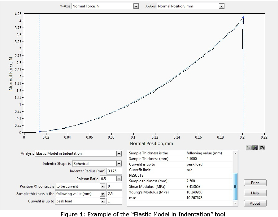
This tool allows for the computing and visualizing of the shear modulus (MPa) and the Youngs modulus (MPa) from an indentation test performed using a spherical indenter.
This model is well adapted for the mechanical characterization of samples (with critical diameter (width) at least 5 times the indenter diameter) bonded on a flat rigid support (at least 10 times stiffer than the sample). For example, any sheet of material lying on a rigid chamber base (limited sliding at the interface can be assumed) or a cartilage layer attached to a thick sub-chondral bone. A user license is required to obtain the results of the elastic model in indentation (Software Add-On MA725, contact Biomomentum to obtain your license).
This model is well adapted for the mechanical characterization of samples (with critical diameter (width) at least 5 times the indenter diameter) bonded on a flat rigid support (at least 10 times stiffer than the sample). For example, any sheet of material lying on a rigid chamber base (limited sliding at the interface can be assumed) or a cartilage layer attached to a thick sub-chondral bone. A user license is required to obtain the results of the elastic model in indentation (Software Add-On MA725, contact Biomomentum to obtain your license).
Results analysis is performed considering the indentation mechanics of an infinitely wide elastic layer bonded to a rigid half-space which has been developed as a model for the layered geometry of cartilage and subchondral bone (Hayes et al., 1972).
How is this model related to the Hertz model?
The Hayes model can directly be related to the Hertz model and both can be used with the “Elastic Model in Indentation” software add-on. To use the Hertz model, set the “Sample thickness is the” parameter to “following value (mm)” and enter a value which is magnitudes larger than the indenter radius (e.g. 99999). Doing so will approximate the thickness to be infinite.
Derivation of Hertz and Hayes model relation with extracts from: Hayes WC, Keer LM, Herrmann G and Mockros LF (1972) A Mathematical Analysis for Indentation Tests of Articular Cartilage. J Biomechanics, Vol. 5, pp. 541-551.Using equations 29:and 30:Where,The Young’s Modulus E is computed from the Shear Modulus with the following equation:By rearranging equations 29 and 30 and using the equation relating the Young’s Modulus to the shear Modulus, the following equation can be obtained:And rearranging this equation:Table 2 is used to obtain values for the spherical indenter:As an example, using an estimated contact region (a) of 1mm and a sample 2mm in thickness (h), the correction factor used would be a/h = 0.5. In this situation, the above equation would become (assuming a Poisson’s Ratio of 0.5 and using Table 2):On the other hand, the Hertz Model would assume an infinite thickness for the measurement of the contact area such that a/h tends toward 0 resulting in the following equation:The Mach-1 Analysis software inputs a K = 2/3 and a χ = 1 as a limiting case when the ratio a/h tends toward zero (assumed infinite thickness). In this situation, the Hayes model becomes equivalent to the Hertz’s Model:
On which types of samples can I use the Hayes model to determine the elastic modulus?
Any elastic sample that is a locally uniform thickness (within approximately 0.1mm). For example: skin, hydrogel, intervertebral disk, cartilage, brain tissue, meniscus, rubber/elastomer, demineralized teeth/shell, tissue phantoms, biocoatings, elastic adhesives, ovary, iris, tendon/ligaments, foam, etc.
This model is unideal for very high modulus samples if they do not elastically deform and simply plastically deform (fracture) under indentation. Slightly less than high modulus samples can still be analyzed with this model as long as only the initial section of the curve is used to fit the model (e.g. 0 to 5um indentation amplitude). You must assume that this first section is elastic.
How is the raw Force vs Displacement curve used to determine the modulus?
Equation 29 and the lookup table are used iteratively until an appropriate relationship between a/h and χ is found. Then, the new a/h ratio is used to find the variable K in the lookup table. This iteration is performed for each indentation depth (w0).
Equation 30 can be rearranged into a form of y=mx. In this form: y = force (P), m = shear modulus (G) and x is the rest:
Using the variable K, the Poisson's ratio (v), the depth at each point (w0), the sample thickness (h) and the indenter radius (R), the slope (G) can be found by plotting y vs x.
Once plotted, the variables can be visualized as follows:
Finally, the Young’s Modulus E is computed from the Shear Modulus G with the following equation:
Related Articles
Questions and Answers regarding Spherical Indentation of Cartilage
Is there a suggested Poisson's ratio to use when analyzing indentations? If an indentation is performed in 1 second or less, it can normally be considered "instantaneous" and a Poisson's ratio of 0.5 should be used (i.e. the liquid inside the sample ...Low-Pass Filter Questions
NOTE: THIS HAS BEEN SOLVED IN VERSION 4.4.0.29 BY APPLYING THE FILTER TO BOTH LOAD AND POSITION CHANNELS. In the "Load Cells" menu, the Low-Pass Filter can be activated or deactivated. Some common values are 3rd order 5Hz cutoff and 3rd order 20Hz ...Main differences when using a spherical vs cylindrical indenters
Here are the main differences when using a spherical vs cylindrical indenter: Spherical Shaped Indenter Cylindrical Shaped Indenter A model should be used to fit to this data (Hayes, Hertz, Sneddon). See Mach-1 Analysis User Manual for more ...DAQmx Self-Test (Error: -88705)
NOTE: in Mach-1 Motion version 4.5.0.1+ (ESP302), the software will automatically search through all DAQ ports. The method below is not necessary. This error is usually caused by having an incorrect DAQ# in the Mach-1 Motion configuration file. ...Load Cell Handling
It is important to be knowledgeable about your load cell before handling such a sensitive device. Please view the following video for basic tips on handling: https://youtu.be/ah3yxFmwBas Another particularity of single-axis load cells is that the ...